User Guide
Background of PCSE
Crop models in Wageningen
The Python Crop Simulation Environment was developed because of a need to re-implement crop simulation models that were developed in Wageningen. Many of the Wageningen crop simulation models were originally developed in FORTRAN77 or using the FORTRAN Simulation Translator (FST). Although this approach has yielded high quality models with high numerical performance, the inherent limitations of models written in FORTRAN is also becoming increasingly evident:
The structure of the models is often rather monolithic and the different parts are very tightly coupled. Replacing parts of the model with another simulation approach is not easy.
The models rely on file-based I/O which is difficult to change. For example, interfacing with databases is complicated in FORTRAN.
In general, with low-level languages like FORTRAN, simple things already take many lines of code and mistakes are easily made, particularly by agronomists and crop scientist that have limited experience in developing or adapting software.
To overcome many of the limitations above, the Python Crop Simulation Environment (PCSE) was developed. It provides an environment for developing simulation models as well as a number of implementations of crop simulation models. PCSE is written in pure Python code which makes it more flexible, easier to modify and extensible allowing easy interfacing with databases, graphical user interfaces, visualization tools and numerical/statistical packages. PCSE has several interesting features:
Implementation in pure Python. The core system has a small number of dependencies outside the Python standard library. However many data providers require certain packages to be installed. Most of these can be automatically installed from the Python Package Index (PyPI) (SQLAlchemy, PyYAML, openpyxl, requests) and in processing of the output of models is most easily done with pandas DataFrames.
Modular design allowing you to add or change components relatively quickly with a simple but powerful approach to communicate variables between modules.
Similar to FST, it enforces good model design by explicitly separating parameters, rate variables and state variables. Moreover PCSE takes care of the module initialization, calculation of rates of changes, updating of state variables and actions needed to finalize the simulation.
Input/Output is completely separated from the simulation model itself. Therefore PCSE models can easily read from and write to text files, databases and scientific formats such as HDF or NetCDF. Moreover, PCSE models can be easily embedded in, for example, docker containers to build a web API around a crop model.
Built-in testing of program modules ensuring integrity of the system
Why Python
PCSE was first and foremost developed from a scientific need, to be able to quickly adapt models and test ideas. In science, Python is quickly becoming a tool for implementing algorithms, visualization and explorative analysis due to its clear syntax and ease of use. An additional advantage is that the C implementation of Python can be easily interfaced with routines written in FORTRAN and therefore many FORTRAN routines can be reused by simulation models written with PCSE.
Many packages exist for numeric analysis (e.g. NumPy, SciPy), visualisation (e.g. MatPlotLib, Chaco), distributed computing (e.g. IPython, pyMPI) and interfacing with databases (e.g. SQLAlchemy). Moreover, for statistical analyses an interface with R-project can be established through Rpy or Rserve. Finally, Python is an Open Source interpreted programming language that runs on almost any hardware and operating system.
Given the above considerations, it was quickly recognized that Python was a good choice. Although, PCSE was developed for scientific purposes, it has already been implemented for tasks in production environments and has been embedded in container-based web services.
History of PCSE
Up until version 4.1, PCSE was called “PyWOFOST” as its primary goal was to provide a Python implementation of the WOFOST crop simulation model. However, as the system has grown it has become evident that the system can be used to implement, extend or hybridize (crop) simulation models. Therefore, the name “PyWOFOST” became too narrow and the name Python Crop Simulation Environment was selected in analog with the FORTRAN Simulation Environment (FSE).
Limitations of PCSE
PCSE also has its limitations, in fact there are several:
Speed: flexibility comes a at a price; PCSE is considerably slower than equivalent models written in FORTRAN or another compiled language.
The simulation approach in PCSE is currently limited to rectangular (Euler) integration with a fixed daily time-step. Although the internal time-step of modules can be made more fine-grained if needed.
No graphical user interface. However the lack of a user interface is partly compensated by using PCSE with the pandas package and the Jupyter notebook. PCSE output can be easily converted to a pandas DataFrame which can be used to display charts in an Jupyter notebook. See also my collection of notebooks with examples using PCSE
License
The source code of PCSE is made available under the European Union Public License (EUPL), Version 1.2 or as soon they will be approved by the European Commission - subsequent versions of the EUPL (the “Licence”). You may not use this work except in compliance with the Licence. You may obtain a copy of the Licence at: https://joinup.ec.europa.eu/community/eupl/og_page/eupl
The PCSE package contains some modules that have been taken and/or modified from other open source projects:
the pydispatch module obtained from http://pydispatcher.sourceforge.net/ which is distributed under a BSD style license.
The traitlets module which was taken and adapted from the IPython project (https://ipython.org/) which are distributed under a BSD style license. A PCSE specific version of traitlets was created and is available here
See the project pages of both projects for exact license terms.
Installing PCSE
Requirements and dependencies
PCSE is being developed on Ubuntu Linux 18.04 and Windows 10 using python 3.9 and python 3.10 As Python is a platform independent language, PCSE works equally well on Linux, Windows or Mac OSX. Before installing PCSE, Python itself must be installed on your system which we will demonstrate below. PCSE has a number of dependencies on other python packages which are the following:
- SQLAlchemy<2.0
- PyYAML>=3.11
- openpyxl>=3.0
- requests>=2.0.0
- pandas>=0.20
- traitlets-pcse==5.0.0.dev
The last package in the list is a modified version of the traitlets package which provides some additional functionality used by PCSE.
Setting up your python environment
A convenient way to set up your python environment for PCSE is through the Anaconda python distribution. In the present PCSE Documentation all examples of installing and using PCSE refer to the Windows 10 platform.
First, we suggest you download and install the MiniConda python distribution which provides a minimum
python environment that we will use to bootstrap a dedicated environment for PCSE. For the rest
of this guide we will assume that you use Windows 10 and install the
64bit miniconda for python 3 (Miniconda3-latest-Windows-x86_64.exe). The environment that
we will create contains not only the dependencies for PCSE, it also includes many other useful packages
such as IPython, `Pandas`_ and the Jupyter notebook. These packages will be used in the Getting Started section
as well.
After installing MiniConda you should open a command box and check that conda is installed properly:
(base) C:\>conda info

     active environment : base
    active env location : C:\data\Miniconda3
            shell level : 1
       user config file : C:\Users\wit015\.condarc
 populated config files : C:\Users\wit015\.condarc
          conda version : 23.11.0
    conda-build version : not installed
         python version : 3.8.18.final.0
                 solver : libmamba (default)
       virtual packages : __archspec=1=x86_64
                          __conda=23.11.0=0
                          __win=0=0
       base environment : C:\data\Miniconda3  (writable)
      conda av data dir : C:\data\Miniconda3\etc\conda
  conda av metadata url : None
           channel URLs : https://conda.anaconda.org/conda-forge/win-64
                          https://conda.anaconda.org/conda-forge/noarch
                          https://repo.anaconda.com/pkgs/main/win-64
                          https://repo.anaconda.com/pkgs/main/noarch
                          https://repo.anaconda.com/pkgs/r/win-64
                          https://repo.anaconda.com/pkgs/r/noarch
                          https://repo.anaconda.com/pkgs/msys2/win-64
                          https://repo.anaconda.com/pkgs/msys2/noarch
          package cache : C:\data\Miniconda3\pkgs
                          C:\Users\wit015\.conda\pkgs
                          C:\Users\wit015\AppData\Local\conda\conda\pkgs
       envs directories : C:\data\Miniconda3\envs
                          C:\Users\wit015\.conda\envs
                          C:\Users\wit015\AppData\Local\conda\conda\envs
               platform : win-64
             user-agent : conda/23.11.0 requests/2.31.0 CPython/3.8.18 Windows/10 Windows/10.0.19045 solver/libmamba conda-libmamba-solver/23.11.1 libmambapy/1.5.3
          administrator : False
             netrc file : None
           offline mode : False
Now we will use a Conda environment file to recreate the python environment that we use to develop and run
PCSE. First you should download the conda environment file (downloads/py3_pcse.yml).
The environment include the Jupyter notebook and IPython which are
needed for running the getting started section and the example notebooks. Save the environment file
on a temporary location such as d:\temp\make_env\. We will now create a dedicated virtual environment
using the command conda env create and tell conda to use the environment file with the
option -f py3_pcse.yml as show below:
(C:\Miniconda3) D:\temp\make_env>conda env create -f py3_pcse.yml
Fetching package metadata .............
Solving package specifications: .
intel-openmp-2 100% |###############################| Time: 0:00:00   6.39 MB/s

... Lots of output here

Installing collected packages: traitlets-pcse
Successfully installed traitlets-pcse-5.0.0.dev0
#
# To activate this environment, use:
# > activate py3_pcse
#
# To deactivate an active environment, use:
# > deactivate
#
# * for power-users using bash, you must source
#
You can then activate your environment (note the addition of (py3_pcse) on your command prompt):
D:\temp\make_env>conda activate py3_pcse
Deactivating environment "C:\Miniconda3"...
Activating environment "C:\Miniconda3\envs\py3_pcse"...

(py3_pcse) D:\temp\make_env>
Installing PCSE
The easiest way to install PCSE is through the python package index (PyPI). Installing from PyPI is mostly useful if you are interested in using the functionality provided by PCSE in your own scripts, but are not interested in modifying or contributing to PCSE itself. Installing from PyPI is done using the package installer pip which searches the python package index for a package, downloads and installs it into your python environment (example below for PCSE 6.0.0):
(py3_pcse) D:\temp\make_env>pip install pcse

Collecting pcse
  Downloading https://files.pythonhosted.org/packages/8c/92/d4444cce1c58e5a96f4d6dc9c0e042722f2136df24a2750352e7eb4ab053/PCSE-5.4.0.tar.gz (791kB)
    100% |¦¦¦¦¦¦¦¦¦¦¦¦¦¦¦¦¦¦¦¦¦¦¦¦¦¦¦¦¦¦¦¦| 798kB 1.6MB/s
Requirement already satisfied: numpy>=1.6.0 in c:\miniconda3\envs\py3_pcse\lib\site-packages (from pcse) (1.15.1)
Requirement already satisfied: SQLAlchemy>=0.8.0 in c:\miniconda3\envs\py3_pcse\lib\site-packages (from pcse) (1.2.11)
Requirement already satisfied: PyYAML>=3.11 in c:\miniconda3\envs\py3_pcse\lib\site-packages (from pcse) (3.13)
Requirement already satisfied: xlrd>=0.9.3 in c:\miniconda3\envs\py3_pcse\lib\site-packages (from pcse) (1.1.0)
Requirement already satisfied: xlwt>=1.0.0 in c:\miniconda3\envs\py3_pcse\lib\site-packages (from pcse) (1.3.0)
Requirement already satisfied: requests>=2.0.0 in c:\miniconda3\envs\py3_pcse\lib\site-packages (from pcse) (2.19.1)
Requirement already satisfied: pandas>=0.20 in c:\miniconda3\envs\py3_pcse\lib\site-packages (from pcse) (0.23.4)
Requirement already satisfied: traitlets-pcse==5.0.0.dev in c:\miniconda3\envs\py3_pcse\lib\site-packages (from pcse) (5.0.0.dev0)
Requirement already satisfied: chardet<3.1.0,>=3.0.2 in c:\miniconda3\envs\py3_pcse\lib\site-packages (from requests>=2.0.0->pcse) (3.0.4)
Requirement already satisfied: idna<2.8,>=2.5 in c:\miniconda3\envs\py3_pcse\lib\site-packages (from requests>=2.0.0->pcse) (2.7)
Requirement already satisfied: certifi>=2017.4.17 in c:\miniconda3\envs\py3_pcse\lib\site-packages (from requests>=2.0.0->pcse) (2018.8.24)
Requirement already satisfied: urllib3<1.24,>=1.21.1 in c:\miniconda3\envs\py3_pcse\lib\site-packages (from requests>=2.0.0->pcse) (1.23)
Requirement already satisfied: python-dateutil>=2.5.0 in c:\miniconda3\envs\py3_pcse\lib\site-packages (from pandas>=0.20->pcse) (2.7.3)
Requirement already satisfied: pytz>=2011k in c:\miniconda3\envs\py3_pcse\lib\site-packages (from pandas>=0.20->pcse) (2018.5)
Requirement already satisfied: six in c:\miniconda3\envs\py3_pcse\lib\site-packages (from traitlets-pcse==5.0.0.dev->pcse) (1.11.0)
Requirement already satisfied: decorator in c:\miniconda3\envs\py3_pcse\lib\site-packages (from traitlets-pcse==5.0.0.dev->pcse) (4.3.0)
Requirement already satisfied: ipython-genutils in c:\miniconda3\envs\py3_pcse\lib\site-packages (from traitlets-pcse==5.0.0.dev->pcse) (0.2.0)
Building wheels for collected packages: pcse
  Running setup.py bdist_wheel for pcse ... done
  Stored in directory: C:\Users\wit015\AppData\Local\pip\Cache\wheels\2f\e6\2c\3952ff951dffea5ab2483892edcb7f9310faa319d050d3be6c
Successfully built pcse
twisted 18.7.0 requires PyHamcrest>=1.9.0, which is not installed.
mkl-random 1.0.1 requires cython, which is not installed.
mkl-fft 1.0.4 requires cython, which is not installed.
Installing collected packages: pcse
Successfully installed pcse-6.0.0
If you want to develop with or contribute to PCSE, than you should fork the PCSE repository on GitHub and get a local copy of PCSE using git clone. See the help on github and for Windows/Mac users the GitHub Desktop application.
Testing PCSE
To guarantee its integrity, the PCSE package includes a limited number of internal tests that are installed automatically with PCSE. In addition, the PCSE git repository has a large number of the tests in the test folder which do a more thorough job in testing but will take a long time to complete (e.g. an hour or more). The internal tests present users with a quick way to ensure that the output produced by the different components matches with the expected outputs. While the full test suite is useful for developers only.
Test data for the internal tests can be found in the pcse.tests.test_data package as well as in an SQLite database (pcse.db). This database can be found under .pcse in your home folder and will be automatically created when importing PCSE for the first time. When you delete the database file manually it will be recreated next time you import PCSE.
For running the internal tests of the PCSE package we need to start python and import pcse:
(py3_pcse) C:\>python
Python 3.10.14 | packaged by conda-forge | (main, Mar 20 2024, 12:40:08) [MSC v.1938 64 bit (AMD64)]
Type 'copyright', 'credits' or 'license' for more information
>>> import pcse
Building PCSE demo database at: C:\Users\wit015\.pcse\pcse.db ... OK
>>>
Next, the tests can be executed by calling the test() function at the top of the package:
>>> pcse.test()
runTest (pcse.tests.test_abioticdamage.Test_FROSTOL) ... ok
runTest (pcse.tests.test_partitioning.Test_DVS_Partitioning) ... ok
runTest (pcse.tests.test_evapotranspiration.Test_PotentialEvapotranspiration) ... ok
runTest (pcse.tests.test_evapotranspiration.Test_WaterLimitedEvapotranspiration1) ... ok
runTest (pcse.tests.test_evapotranspiration.Test_WaterLimitedEvapotranspiration2) ... ok
runTest (pcse.tests.test_respiration.Test_WOFOSTMaintenanceRespiration) ... ok
runTest (pcse.tests.test_penmanmonteith.Test_PenmanMonteith1) ... ok
runTest (pcse.tests.test_penmanmonteith.Test_PenmanMonteith2) ... ok
runTest (pcse.tests.test_penmanmonteith.Test_PenmanMonteith3) ... ok
runTest (pcse.tests.test_penmanmonteith.Test_PenmanMonteith4) ... ok
runTest (pcse.tests.test_agromanager.TestAgroManager1) ... ok
runTest (pcse.tests.test_agromanager.TestAgroManager2) ... ok
runTest (pcse.tests.test_agromanager.TestAgroManager3) ... ok
runTest (pcse.tests.test_agromanager.TestAgroManager4) ... ok
runTest (pcse.tests.test_agromanager.TestAgroManager5) ... ok
runTest (pcse.tests.test_agromanager.TestAgroManager6) ... ok
runTest (pcse.tests.test_agromanager.TestAgroManager7) ... ok
runTest (pcse.tests.test_agromanager.TestAgroManager8) ... ok
runTest (pcse.tests.test_wofost72.TestWaterlimitedGrainMaize) ... ok
runTest (pcse.tests.test_wofost72.TestWaterlimitedPotato) ... ok
runTest (pcse.tests.test_wofost72.TestWaterlimitedWinterRapeseed) ... ok
runTest (pcse.tests.test_wofost72.TestWaterlimitedWinterWheat) ... ok
runTest (pcse.tests.test_wofost72.TestPotentialGrainMaize) ... ok
runTest (pcse.tests.test_wofost72.TestPotentialWinterWheat) ... ok
runTest (pcse.tests.test_wofost72.TestPotentialWinterRapeseed) ... ok
runTest (pcse.tests.test_wofost72.TestWaterlimitedSunflower) ... ok
runTest (pcse.tests.test_wofost72.TestPotentialSpringBarley) ... ok
runTest (pcse.tests.test_wofost72.TestPotentialSunflower) ... ok
runTest (pcse.tests.test_wofost72.TestPotentialPotato) ... ok
runTest (pcse.tests.test_wofost72.TestWaterlimitedSpringBarley) ... ok

----------------------------------------------------------------------
Ran 30 tests in 22.482s

OK
If the model output matches the expected output the test will report ‘OK’, otherwise an error will be produced with a detailed traceback on where the problem occurred. Note that the results may deviate from the output above when tests were added or removed.
Moreover, SQLAlchemy may complain with a warning that can be safely ignored:
C:\Miniconda3\envs\py3_pcse\lib\site-packages\sqlalchemy\sql\sqltypes.py:603: SAWarning:
Dialect sqlite+pysqlite does *not* support Decimal objects natively, and SQLAlchemy must
convert from floating point - rounding errors and other issues may occur. Please consider
storing Decimal numbers as strings or integers on this platform for lossless storage.
Getting started
This guide will help you install PCSE as well as provide some examples to get you started with modelling. The examples are currently focused on applying the WOFOST and LINTUL3 crop simulation models, although other crop simulation models may become available within PCSE in the future.
Note that the examples below are also available as Jupyter notebooks on my github page: https://github.com/ajwdewit/pcse_notebooks
An interactive PCSE/WOFOST session
The easiest way to demonstrate PCSE is to import WOFOST from PCSE and run it from an interactive Python session. We will be using the start_wofost() script that connects to a the demo database which contains meteorologic data, soil data, crop data and management data for a grid location in South-Spain.
Initializing PCSE/WOFOST and advancing model state
Let’s start a WOFOST object for modelling winter-wheat on a location in South-Spain for the year 2000 under water-limited conditions.:
>>> wofost_object = pcse.start_wofost()
>>> type(wofost_object)
<class 'pcse.models.Wofost72_WLP_CWB'>
You have just successfully initialized a PCSE/WOFOST object in the Python interpreter, which is in its initial state and waiting to do some simulation. We can now advance the model state for example with 1 day:
>>> wofost_object.run()
Advancing the crop simulation with only 1 day, is often not so useful so the number of days to simulate can be specified as well:
>>> wofost_object.run(days=10)
Getting information about state and rate variables
Retrieving information about the calculated model states or rates can be done with the get_variable() method on a PCSE object. For example, to retrieve the leaf area index value in the current model state you can do:
>>> wofost_object.get_variable('LAI')
0.28708095263317146
>>> wofost_object.run(days=25)
>>> wofost_object.get_variable('LAI')
1.5281215808337203
Showing that after 11 days the LAI value is 0.287. When we increase time with another 25 days, the LAI increases to 1.528. The get_variable method can retrieve any state or rate variable that is defined somewhere in the model. Finally, we can finish the crop season by letting it run until the model terminates because the crop reaches maturity or the harvest date:
>>> wofost_object.run_till_terminate()
Next we retrieve the simulation results at each time-step (‘output’) of the simulation:
>>> output = wofost_object.get_output()
We can now use the pandas package to turn the simulation output into a
dataframe which is much easier to handle and can be exported to different
file types. For example an excel file which should look like this
downloads/wofost_results.xls:
>>> import pandas as pd
>>> df = pd.DataFrame(output)
>>> df.to_excel("wofost_results.xls")
Finally, we can retrieve the results at the end of the crop cycle (summary results) and have a look at these as well:
>>> summary_output = wofost_object.get_summary_output()
>>> msg = "Reached maturity at {DOM} with total biomass {TAGP} kg/ha "\
"and a yield of {TWSO} kg/ha."
>>> print(msg.format(**summary_output[0]))
Reached maturity at 2000-05-31 with total biomass 15261.7521735 kg/ha and a yield of 7179.80460783 kg/ha.

>>> summary_output
[{'CTRAT': 22.457536342947606,
  'DOA': datetime.date(2000, 3, 28),
  'DOE': datetime.date(2000, 1, 1),
  'DOH': None,
  'DOM': datetime.date(2000, 5, 31),
  'DOS': None,
  'DOV': None,
  'DVS': 2.01745939841335,
  'LAIMAX': 6.132711275237731,
  'RD': 60.0,
  'TAGP': 15261.752173534584,
  'TWLV': 3029.3693107257263,
  'TWRT': 1546.990661062695,
  'TWSO': 7179.8046078262705,
  'TWST': 5052.578254982587}]
Running PCSE/WOFOST with custom input data
For running PCSE/WOFOST (and PCSE models in general) with your own data sources you need three different types of inputs:
Model parameters that parameterize the different model components. These parameters usually consist of a set of crop parameters (or multiple sets in case of crop rotations), a set of soil parameters and a set of site parameters. The latter provide ancillary parameters that are specific for a location.
Driving variables represented by weather data which can be derived from various sources.
Agromanagement actions which specify the farm activities that will take place on the field that is simulated by PCSE.
For the second example we will run a simulation for sugar beet in
Wageningen (Netherlands) and we will read the input data step by step from
several different sources instead of using the pre-configured start_wofost()
script. For the example we will assume that data files are in the directory
D:\userdata\pcse_examples and all the parameter files needed can be
found by unpacking this zip file downloads/quickstart_part2.zip.
First we will import the necessary modules and define the data directory:
>>> import os
>>> import pcse
>>> import matplotlib.pyplot as plt
>>> data_dir = r'D:\userdata\pcse_examples'
Crop parameters
The crop parameters consist of parameter names and the corresponding parameter values that are needed to parameterize the components of the crop simulation model. These are crop-specific values regarding phenology, assimilation, respiration, biomass partitioning, etc. The parameter file for sugar beet is taken from the crop files in the WOFOST Control Centre.
The crop parameters for many models in Wageningen are often provided in the CABO format that could be read with the TTUTIL FORTRAN library. PCSE tries to be backward compatible as much as possible and provides the CABOFileReader for reading parameter files in CABO format. the CABOFileReader returns a dictionary with the parameter name/value pairs:
>>> from pcse.input import CABOFileReader
>>> cropfile = os.path.join(data_dir, 'sug0601.crop')
>>> cropdata = CABOFileReader(cropfile)
>>> print(cropdata)
Printing the cropdata dictionary gives you a listing of the header and all parameters and their values.
Soil parameters
The soildata dictionary provides the parameter name/value pairs related to the soil type and soil physical properties. The number of parameters is variable depending on the soil water balance type that is used for the simulation. For this example, we will use the water balance for freely draining soils and use the soil file for medium fine sand: ec3.soil. This file is also taken from the soil files in the WOFOST Control Centre
>>> soilfile = os.path.join(data_dir, 'ec3.soil')
>>> soildata = CABOFileReader(soilfile)
Site parameters
The site parameters provide ancillary parameters that are not related to the crop or the soil. Examples are the initial conditions of the water balance such as the initial soil moisture content (WAV) and the initial and maximum surface storage (SSI, SSMAX). Also the atmospheric CO2 concentration is a typical site parameter. For the moment, we can define these parameters directly on the Python commandline as a simple python dictionary. However, it is more convenient to use the WOFOST72SiteDataProvider that documents the site parameters and provides sensible defaults:
>>> from pcse.input import WOFOST72SiteDataProvider
>>> sitedata = WOFOST72SiteDataProvider(WAV=100)
>>> print(sitedata)
{'SMLIM': 0.4, 'NOTINF': 0, 'SSI': 0.0, 'SSMAX': 0.0, 'IFUNRN': 0, 'WAV': 100.0}
Finally, we need to pack the different sets of parameters into one variable using the ParameterProvider. This is needed because PCSE expects one variable that contains all parameter values. Using this approach has the additional advantage that parameters value can be easily overridden in case of running multiple simulations with slightly different parameter values:
>>> from pcse.base import ParameterProvider
>>> parameters = ParameterProvider(cropdata=cropdata, soildata=soildata, sitedata=sitedata)
AgroManagement
The agromanagement inputs provide the start date of the agricultural campaign, the start_date/start_type of the crop simulation, the end_date/end_type of the crop simulation and the maximum duration of the crop simulation. The latter is included to avoid unrealistically long simulations for example as a results of a too high temperature sum requirement.
The agromanagement inputs are defined with a special syntax called YAML which allows to easily create more complex structures which is needed for defining the agromanagement. The agromanagement file for sugar beet in Wageningen sugarbeet_calendar.agro can be read with the YAMLAgroManagementReader:
>>> from pcse.input import YAMLAgroManagementReader
>>> agromanagement_file = os.path.join(data_dir, 'sugarbeet_calendar.agro')
>>> agromanagement = YAMLAgroManagementReader(agromanagement_file)
>>> print(agromanagement)
 !!python/object/new:pcse.fileinput.yaml_agro_loader.YAMLAgroManagementReader
 listitems:
 - 2000-01-01:
     CropCalendar:
       crop_name: sugarbeet
       variety_name: sugar_beet_601
       crop_start_date: 2000-04-05
       crop_start_type: emergence
       crop_end_date: 2000-10-20
       crop_end_type: harvest
       max_duration: 300
     StateEvents: null
     TimedEvents: null
Daily weather observations
Daily weather variables are needed for running the simulation. There are several data providers in PCSE for reading weather data, see the section on weather data providers to get an overview.
For this example we will use the weather data from the NASA Power database which provides global weather data with a spatial resolution of 0.5 degree (~50 km). We will retrieve the data from the Power database for the location of Wageningen. Note that it can take around 30 seconds to retrieve the weather data from the NASA Power server the first time:
>>> from pcse.input import NASAPowerWeatherDataProvider
>>> wdp = NASAPowerWeatherDataProvider(latitude=52, longitude=5)
>>> print(wdp)
Weather data provided by: NASAPowerWeatherDataProvider
--------Description---------
NASA/POWER CERES/MERRA2 Native Resolution Daily Data
----Site characteristics----
Elevation:    3.5
Latitude:  52.000
Longitude:  5.000
Data available for 1984-01-01 - 2024-03-20
Number of missing days: 0
Importing, initializing and running a PCSE model
Internally, PCSE uses a simulation engine to run a crop simulation. This engine takes a configuration file that specifies the components for the crop, the soil and the agromanagement that need to be used for the simulation. So any PCSE model can be started by importing the engine and initializing it with a given configuration file and the corresponding parameters, weather data and agromanagement.
However, as many users of PCSE only need a particular configuration (for example the WOFOST model for potential production), preconfigured Engines are provided in pcse.models. For the sugarbeet example we will import the WOFOST model for water-limited simulation using the classic waterbalance. The latter simulates the soil water dynamics assuming a freely draining soil:
>>> from pcse.models import Wofost72_WLP_CWB
>>> wofsim = Wofost72_WLP_CWB(parameters, wdp, agromanagement)
We can then run the simulation and show some final results such as the anthesis and harvest dates (DOA, DOH), total biomass (TAGP) and maximum LAI (LAIMAX). Next, we retrieve the time series of daily simulation output using the get_output() method on the WOFOST object:
>>> wofsim.run_till_terminate()
>>> output = wofsim.get_output()
>>> len(output)
294
As the output is returned as a list of dictionaries, we need to unpack these variables from the list of output:
>>> varnames = ["day", "DVS", "TAGP", "LAI", "SM"]
>>> tmp = {}
>>> for var in varnames:
>>>     tmp[var] = [t[var] for t in output]
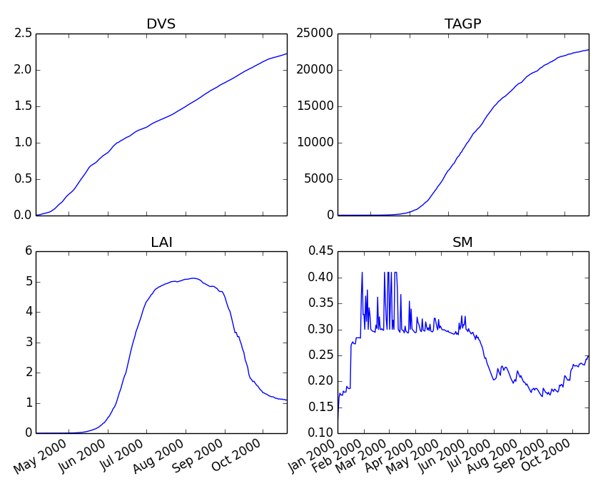
Finally, we can generate some figures of WOFOST variables such as the development (DVS), total biomass (TAGP), leaf area index (LAI) and root-zone soil moisture (SM) using the MatPlotLib plotting package:
>>> day = tmp.pop("day")
>>> fig, axes = plt.subplots(nrows=2, ncols=2, figsize=(10,8))
>>> for var, ax in zip(["DVS", "TAGP", "LAI", "SM"], axes.flatten()):
>>>     ax.plot_date(day, tmp[var], 'b-')
>>>     ax.set_title(var)
>>> fig.autofmt_xdate()
>>> fig.savefig('sugarbeet.png')
This should generate a figure of the simulation results as shown below. The complete Python
script for this examples can be downloaded here downloads/quickstart_demo2.py
Running a simulation with PCSE/LINTUL3
The LINTUL model (Light INTerception and UtiLisation) is a simple generic crop model, which simulates dry matter production as the result of light interception and utilization with a constant light use efficiency. In PCSE the LINTUL family of models has been implemented including the LINTUL3 model which is used for simulation of crop production under water-limited and nitrogen-limited conditions.
For the third example, we will use LINTUL3 for simulating spring-wheat in the Netherlands under water-limited
and nitrogen-limited conditions. We will again assume that data files are in the directory
D:\userdata\pcse_examples and all the parameter files needed can be
found by unpacking this zip file downloads/quickstart_part3.zip. Note that this guide is also available
as an IPython notebook: downloads/running_LINTUL3.ipynb.
First we will import the necessary modules and define the data directory. We also assume that you have the matplotlib, `pandas`_ and PyYAML packages installed on your system.:
>>> import os
>>> import pcse
>>> import matplotlib.pyplot as plt
>>> import pandas as pd
>>> import yaml
>>> data_dir = r'D:\userdata\pcse_examples'
Similar to the previous example, for running the PCSE/LINTUL3 model we need to define the tree types of inputs (parameters, weather data and agromanagement).
Reading model parameters
Model parameters can be easily read from the input files using the PCSEFileReader as we have seen in the previous example:
>>> from pcse.input import PCSEFileReader
>>> crop = PCSEFileReader(os.path.join(data_dir, "lintul3_springwheat.crop"))
>>> soil = PCSEFileReader(os.path.join(data_dir, "lintul3_springwheat.soil"))
>>> site = PCSEFileReader(os.path.join(data_dir, "lintul3_springwheat.site"))
However, PCSE models expect a single set of parameters and therefore they need to be combined using the ParameterProvider:
>>> from pcse.base import ParameterProvider
>>> parameterprovider = ParameterProvider(soildata=soil, cropdata=crop, sitedata=site)
Reading weather data
For reading weather data we will use the ExcelWeatherDataProvider. This WeatherDataProvider uses nearly the same file format as is used for the CABO weather files but stores its data in an MicroSoft Excel file which makes the weather files easier to create and update:
>>> from pcse.input import ExcelWeatherDataProvider
>>> weatherdataprovider = ExcelWeatherDataProvider(os.path.join(data_dir, "nl1.xlsx"))
>>> print(weatherdataprovider)
Weather data provided by: ExcelWeatherDataProvider
--------Description---------
Weather data for:
Country: Netherlands
Station: Wageningen, Location Haarweg
Description: Observed data from Station Haarweg in Wageningen
Source: Meteorology and Air Quality Group, Wageningen University
Contact: Peter Uithol
----Site characteristics----
Elevation:    7.0
Latitude:  51.970
Longitude:  5.670
Data available for 2004-01-02 - 2008-12-31
Number of missing days: 32
Defining agromanagement
Defining agromanagement needs a bit more explanation because agromanagement is a relatively complex piece of PCSE. The agromanagement definition for PCSE is written in a format called YAML and for the current example looks like this:
Version: 1.0.0
AgroManagement:
- 2006-01-01:
    CropCalendar:
        crop_name: wheat
        variety_name: spring-wheat
        crop_start_date: 2006-03-31
        crop_start_type: emergence
        crop_end_date: 2006-08-20
        crop_end_type: earliest
        max_duration: 300
    TimedEvents:
    -   event_signal: apply_n
        name:  Nitrogen application table
        comment: All nitrogen amounts in g N m-2
        events_table:
        - 2006-04-10: {amount: 10, recovery: 0.7}
        - 2006-05-05: {amount:  5, recovery: 0.7}
    StateEvents: null
The agromanagement definition starts with Version: indicating the version number of the agromanagement file while the actual definition starts after the label AgroManagement:. Next a date must be provided which sets the start date of the campaign (and the start date of the simulation). Each campaign is defined by zero or one CropCalendars and zero or more TimedEvents and/or StateEvents. The CropCalendar defines the crop name, variety_name, date of sowing, date of harvesting, etc. while the Timed/StateEvents define actions that are either connected to a date or to a model state.
In the current example, the campaign starts on 2006-01-01, there is a crop calendar for spring-wheat starting on 2006-03-31 with a harvest date of 2006-08-20 or earlier if the crop reaches maturity before this date. Next there are timed events defined for applying N fertilizer at 2006-04-10 and 2006-05-05. The current example has no state events. For a thorough description of all possibilities see the section on AgroManagement in the Reference Guide (Chapter 3).
Loading the agromanagement definition must by done with the YAMLAgroManagementReader:
>>> from pcse.input import YAMLAgroManagementReader
>>> agromanagement = YAMLAgroManagementReader(os.path.join(data_dir, "lintul3_springwheat.amgt"))
>>> print(agromanagement)
!!python/object/new:pcse.fileinput.yaml_agro_loader.YAMLAgroManagementReader
listitems:
- 2006-01-01:
    CropCalendar:
      crop_end_date: 2006-10-20
      crop_end_type: earliest
      crop_name: wheat
      variety_name: spring-wheat
      crop_start_date: 2006-03-31
      crop_start_type: emergence
      max_duration: 300
    StateEvents: null
    TimedEvents:
    - comment: All nitrogen amounts in g N m-2
      event_signal: apply_n
      events_table:
      - 2006-04-10:
          amount: 10
          recovery: 0.7
      - 2006-05-05:
          amount: 5
          recovery: 0.7
      name: Nitrogen application table
Starting and running the LINTUL3 model
We have now all parameters, weather data and agromanagement information available to start the LINTUL3 model:
>>> from pcse.models import LINTUL3
>>> lintul3 = LINTUL3(parameterprovider, weatherdataprovider, agromanagement)
>>> lintul3.run_till_terminate()
Next, we can easily get the output from the model using the get_output() method and turn it into a pandas DataFrame:
>>> output = lintul3.get_output()
>>> df = pd.DataFrame(output).set_index("day")
>>> df.tail()
                 DVS       LAI     NUPTT       TAGBM     TGROWTH  TIRRIG  \
day
2006-07-28  1.931748  0.384372  4.705356  560.213626  626.053663       0
2006-07-29  1.953592  0.368403  4.705356  560.213626  626.053663       0
2006-07-30  1.974029  0.353715  4.705356  560.213626  626.053663       0
2006-07-31  1.995291  0.339133  4.705356  560.213626  626.053663       0
2006-08-01  2.014272  0.326169  4.705356  560.213626  626.053663       0

               TNSOIL  TRAIN  TRAN  TRANRF  TRUNOF      TTRAN        WC  \
day
2006-07-28  11.794644  375.4     0       0       0  71.142104  0.198576
2006-07-29  11.794644  376.3     0       0       0  71.142104  0.197346
2006-07-30  11.794644  376.3     0       0       0  71.142104  0.196293
2006-07-31  11.794644  381.6     0       0       0  71.142104  0.198484
2006-08-01  11.794644  381.7     0       0       0  71.142104  0.197384

                 WLVD       WLVG        WRT         WSO         WST
day
2006-07-28  88.548865  17.687197  16.649830  184.991591  268.985974
2006-07-29  89.284828  16.951234  16.150335  184.991591  268.985974
2006-07-30  89.962276  16.273785  15.665825  184.991591  268.985974
2006-07-31  90.635216  15.600845  15.195850  184.991591  268.985974
2006-08-01  91.233828  15.002234  14.739974  184.991591  268.985974
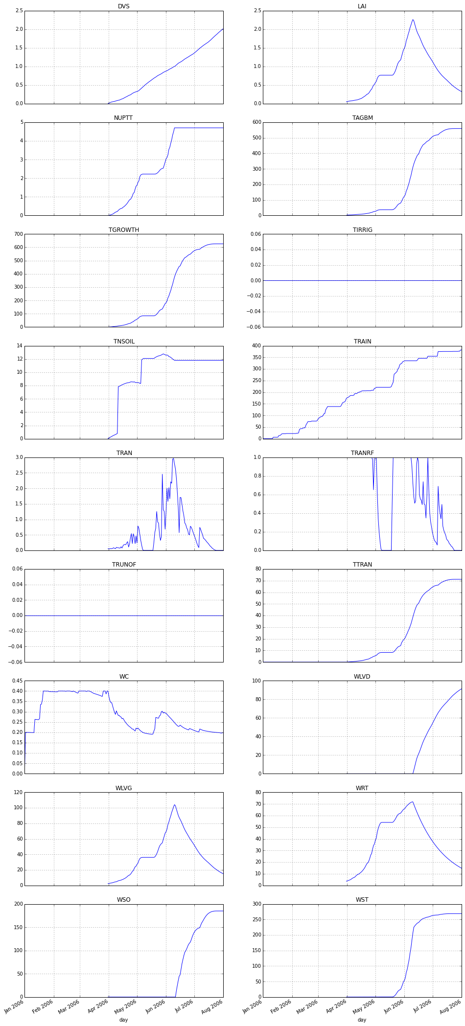
Finally, we can visualize the results from the pandas DataFrame with a few commands if your environment supports plotting:
>>> fig, axes = plt.subplots(nrows=9, ncols=2, figsize=(16,40))
>>> for key, axis in zip(df.columns, axes.flatten()):
>>>     df[key].plot(ax=axis, title=key)
>>> fig.autofmt_xdate()
>>> fig.savefig(os.path.join(data_dir, "lintul3_springwheat.png"))
Advanced topics
Many more examples plus demonstrations of advanced topics are available as Jupyter notebooks at https://github.com/ajwdewit/pcse_notebooks