Reference Guide
An overview of PCSE
The Python Crop Simulation Environment builds on the heritage provided by the earlier approaches developed in Wageningen, notably the Fortran Simulation Environment. The FSE manual (van Kraalingen, 1995) provides a very good overview on the principles of Euler integration and its application to crop simulation models. Therefore, we will not discuss this in detail here.
Nevertheless, PCSE also tries to improve on these approaches by separating the simulation logic into a number of distinct components that play a role in the implementation of (crop) simulation models:
The dynamic part of the simulation is taken care of by a dedicated simulation Engine which handles the initialization, the ordering of rate/state updates for the soil and plant modules as well as keeping track of time, retrieving weather data and calling the agromanager module.
Solving the differential equations for soil/plant system and updating the model state is deferred to SimulationObjects that implement (bio)physical processes such as phenological development or CO2 assimilation.
An AgroManager module is included which takes care of signalling agricultural management actions such as sowing, harvesting, irrigation, etc.
Communication between PCSE components is implemented by either exporting variables into a shared state object or by implementing signals that can be broadcasted and received by any PCSE object.
Several tools are available for providing weather data and reading parameter values from files or databases.
Next, an overview of the different components in PCSE will be provided.
The Engine
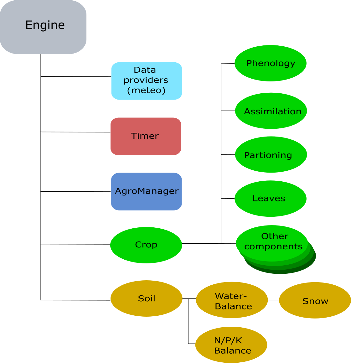
The PCSE Engine provides the environment where the simulation takes place. The engine takes care of reading the model configuration, initializing model components, driving the simulation forward by calling the SimulationObjects, calling the agromanagement unit, keeping track of time, providing the weather data needed and storing the model variables during the simulation for later output. The Engine itself is generic and can be used for any model that is defined in PCSE. The overall structure of the engine can be found in the figure below which shows the different elements that are called by the Engine.
Continuous simulation in PCSE
To implement continuous simulation, the engine uses the same approach as FSE: Euler integration with a fixed time step of one day. The following figure shows the principle of continuous simulation and the execution order of various steps.
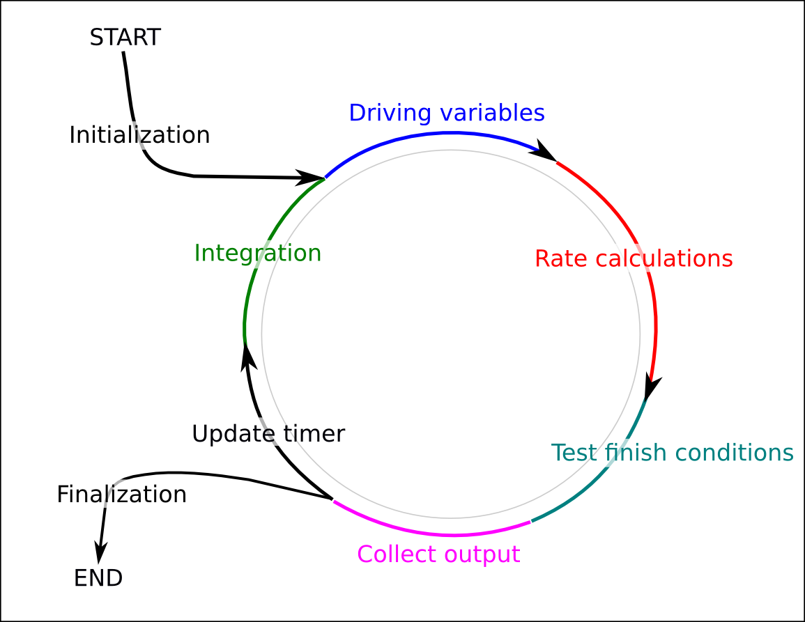
Order of calculations for continuous simulation using Euler integration (after Van Kraalingen, 1995).
The steps in the process cycle that are shown in the figure above are implemented in the simulation Engine which is completely separated from the model logic itself. Moreover, it demonstrates that before the simulation can start the engine has to be initialized which involves several steps:
The model configuration must be loaded;
The AgroManager module must be initialized and called to determine the first and last of the simulation sequence;
The timer must be initialized with the first and last day of the simulation sequence;
The soil component specified in the model configuration must be initialized.
The weather variables must be retrieved for the starting day;
The AgroManager must be called to trigger any management events that are scheduled for the starting day.
The initial rates of change based on the initial states and driving variables must be calculated;
Finally, output can be collected to save the initial states and rates of the simulation.
The next cycle in the simulation will now start with an update of the timer to the next time step (e.g. day). Next, the rates of change of the previous day will be integrated onto the state variables and the driving variables for the current day will be retrieved. Finally, the rates of change will be recalculated based on the new driving variables and updated model states and so forth.
The simulation loop will terminate when some finish condition has been reached. Usually, the AgroManager module will encounter the end of the agricultural campaign and will broadcast a terminate signal that terminates the entire simulation.
Input needed by the Engine
To start the Engine four inputs are needed:
A weather data provider that provides the Engine with the daily values of weather variables. See the section on Weather data providers for an overview of the different options for providing weather data.
A set of parameters that is needed to parameterize the SimulationObjects that simulate the soil and crop processes. Model parameters can be retrieved from different sources like files or databases. PCSE uses three sets of model parameters: crop parameters, soil parameters and site parameters. The latter present an ancillary set of parameters that are not related to the soil or the crop. The atmospheric CO2 concentration is a typical example of a site parameter. Despite having three sets of parameters, all parameters are encapsulated using a ParameterProvider that provides a uniform interface to access the different parameter sets. See the section on Data providers for parameter values for an overview.
Agromanagement information that is needed to schedule agromanagement actions that are taking place during the simulation. See the sections on The AgroManager and Data providers for agromanagement for a detailed overview.
A configuration file that tells the Engine the details of the simulation such as the components to use for the simulation of the crop, the soil and the agromanagement. Moreover, the results that should be stored as final and intermediate outputs and some other details.
Engine configuration files
The engine needs a configuration file that specifies which components should be used for simulation and additional information. This is most easily explained by an example such as the configuration file for the WOFOST 7.2 model for potential crop production:
# -*- coding: utf-8 -*-
# Copyright (c) 2004-2021 Wageningen Environmental Research
# Allard de Wit (allard.dewit@wur.nl), August 2021
"""PCSE configuration file for WOFOST 7.2 Potential Production simulation

This configuration file defines the soil and crop components that
should be used for potential production simulation.
"""

from pcse.soil.classic_waterbalance import WaterbalancePP
from pcse.crop.wofost72 import Wofost72
from pcse.agromanager import AgroManager

# Module to be used for water balance
SOIL = WaterbalancePP

# Module to be used for the crop simulation itself
CROP = Wofost72

# Module to use for AgroManagement actions
AGROMANAGEMENT = AgroManager

# variables to save at OUTPUT signals
# Set to an empty list if you do not want any OUTPUT
OUTPUT_VARS = ["DVS","LAI","TAGP", "TWSO", "TWLV", "TWST",
               "TWRT", "TRA", "RD", "SM", "WWLOW"]
# interval for OUTPUT signals, either "daily"|"dekadal"|"monthly"|"weekly"
# For daily output you change the number of days between successive
# outputs using OUTPUT_INTERVAL_DAYS. For dekadal and monthly
# output this is ignored.
OUTPUT_INTERVAL = "daily"
OUTPUT_INTERVAL_DAYS = 1
# Weekday: Monday is 0 and Sunday is 6
OUTPUT_WEEKDAY = 0

# Summary variables to save at CROP_FINISH signals
# Set to an empty list if you do not want any SUMMARY_OUTPUT
SUMMARY_OUTPUT_VARS = ["DVS","LAIMAX","TAGP", "TWSO", "TWLV", "TWST",
                       "TWRT", "CTRAT", "RD", "DOS", "DOE", "DOA",
                       "DOM", "DOH", "DOV", "CEVST"]

# Summary variables to save at TERMINATE signals
# Set to an empty list if you do not want any TERMINAL_OUTPUT
TERMINAL_OUTPUT_VARS = []
As you can see, the configuration file is written in plain python code. First of all, it defines the placeholders SOIL, CROP and AGROMANAGEMENT that define the components that should be used for the simulation of these processes. These placeholders simply point to the modules that were imported at the start of the configuration file.
Note
Modules in configuration files must be imported using fully qualified names and relative imports cannot be used.
The second part is for defining the variables (OUTPUT_VARS) that should be stored during the model run (during OUTPUT signals) and the details of the regular output interval. Next, summary output SUMMARY_OUTPUT_VARS can be defined that will be generated at the end of each crop cycle. Finally, output can be collected at the end of the entire simulation (TERMINAL_OUTPUT_VARS).
Note
Model configuration files for models that are included in the PCSE package reside in the ‘conf/’ folder inside the package. When the Engine is started with the name of a configuration file, it searches this folder to locate the file. This implies that if you want the start the Engine with your own (modified) configuration file, you must specify it as an absolute path otherwise the Engine will not find it.
The relationship between models and the engine
Models are treated together with the Engine, because models are simply pre-configured Engines. Any model can be started by starting the Engine with the appropriate configuration file. The only difference is that models can have methods that deal with specific characteristics of a model. This kind of functionality cannot be implemented in the Engine because the model details are not known beforehand.
SimulationObjects
PCSE uses SimulationObjects to group parts of the crop simulation model that form a logical entity into separate program code sections. In this way the crop simulation model is grouped into sections that implement certain biophysical processes such as phenology, assimilation, respiration, etc. Simulation objects can be grouped to form components that perform the simulation of an entire crop or a soil profile.
This approach has several advantages:
Model code with a certain purpose is grouped together, making it easier to read, understand and maintain.
A SimulationObject contains only parameters, rate and state variables that are needed. In contrast, with monolythic code it is often unclear (at first glance at least) what biophysical process they belong to.
Isolation of process implementations creates less dependencies, but more importantly, dependencies are evident from the code which makes it easier to modify individual SimulationObjects.
SimulationObjects can be tested individually by comparing output vs the expected output (e.g. unit testing).
SimulationObjects can be exchanged for other objects with the same purpose but a different biophysical approach. For example, the WOFOST assimilation approach could be easily replaced by a more simple Light Use Efficiency or Water Use Efficiency approach, by replacing the SimulationObject that handles the CO2 assimilation.
Characteristics of SimulationObjects
Each SimulationObject is defined in the same way and has a couple of standard sections and methods which facilitates understanding and readability. Each SimulationObject has parameters to define the mathematical relationships, it has state variables to define the state of the system and it has rate variables that describe the rate of change from one time step to the next. Moreover, a SimulationObject may contain other SimulationObjects that together form a logical structure. Finally, the SimulationObject must implement separate code sections for initialization, rate calculation and integration of the rates of change. A finalization step which is called at the end of the simulation can be added optionally.
The skeleton of a SimulationObject looks like this:
class CropProcess(SimulationObject):

    class Parameters(ParamTemplate):
        PAR1 = Float()
        # more parameters defined here

    class StateVariables(StatesTemplate):
        STATE1 = Float()
        # more state variables defined here

    class RateVariables(RatesTemplate):
        RATE1 = Float()
        # more rate variables defined here

    def initialize(self, day, kiosk, parametervalues):
        """Initializes the SimulationObject with given parametervalues."""
        self.params = self.Parameters(parametervalues)
        self.rates = self.RateVariables(kiosk)
        self.states = self.StateVariables(kiosk, STATE1=0., publish=["STATE1"])

    @prepare_rates
    def calc_rates(self, day, drv):
        """Calculate the rates of change given the current states and driving
        variables (drv)."""

        # simple example of rate calculation using rainfall (drv.RAIN)
        self.rates.RATE1 = self.params.PAR1 * drv.RAIN

    @prepare_states
    def integrate(self, day, delt):
        """Integrate the rates of change on the current state variables
        multiplied by the time-step
        """
        self.states.STATE1 += self.rates.RATE1 * delt

    @prepare_states
    def finalize(self, day):
        """do some final calculations when the simulation is finishing."""
The strict separation of program logic was copied from the Fortran Simulation Environment (FSE, Rappoldt and Van Kraalingen 1996 and Van Kraalingen 1995) and is critical to ensure that the simulation results are correct. The different calculations types (integration, driving variables and rate calculations) should be strictly separated. In other words, first all states should be updated, subsequently all driving variables should be calculated, after which all rates of change should be calculated. If this rule is not applied rigorously, some rates may pertain to states at the current time whereas others will pertain to states from the previous time step. Compared to the FSE system and the FORTRAN implementation of WOFOST, the initialize(), calc_rates(), integrate() and finalize() sections match with the ITASK numbers 1, 2, 3, 4.
A complicating factor that arises when using modular code is how to arrange the communication between SimulationObjects. For example, the evapotranspiration SimulationObject will need information about the leaf area index from the leaf_dynamics SimulationObject to calculate the crop transpiration values. In PCSE the communication between SimulationObjects is taken care of by the so-called VariableKiosk. The metaphore kiosk is used because the SimulationObjects publish their rate and/or state variables (or a subset) into the kiosk, other SimulationObjects can subsequently request the variable value from the kiosk without any knowledge about the SimulationObject that published it. Therefore, the VariableKiosk is shared by all SimulationObjects and must be provided when SimulationObjects initialize.
See the section on Exchanging data between model components for a detailed description of the variable kiosk and other ways to communicate between model components.
Simulation Parameters
Usually SimulationObjects have one or more parameters which should be defined as a subclass of the ParamTemplate class. Although parameters can be specified as part of the SimulationObject definition directly, subclassing them from ParamTemplate has a few advantages. First of all, parameters must be initialized and a missing parameter will lead to an exception being raised with a clear message. Secondly, parameters are initialized as read-only attributes which cannot be changed during the simulation. So occasionally overwriting a parameter value is impossible this way.
The model parameters are initialized by the calling the Parameters class definition and providing a dictionary with key/value pairs to define the parameters.
State/Rate variables
The definitions for state and rate variables share many properties. Definitions of rate and state variables should be defined as attributes of a class that inherit from RatesTemplate and StatesTemplate respectively. Names of rate and state variables that are defined this way must be unique across all model components and a duplicate variable name somewhere across the model composition will lead to an exception.
Both class instances need the VariableKiosk as its first input parameter which is needed to register the variables defined. Moreover, variables can be published with the publish keyword as is done in the example above for STATE1. Publishing a variable means that it will be available in the VariableKiosk and can be retrieved by other components based on the name of the variables. The main difference between a rates and a states class is that the states class requires you to provide the initial value of the state as a keyword parameter in the call. Failing to provide the initial value will lead to an exception being raised.
Instances of objects containing rate and state variables are read-only by default. In order to change the value of a rate or state, the instance must be unlocked. For this purpose the decorators @prepare_rates and @prepare_states are being placed in front of the calls to calc_rates() and integrate() which take care of unlocking and locking the states and rates instances. Using this approach rate variables can only be changed during the call where the rates are calculated, states variables are read-only at that stage. Similarly, state variables can only be changed during the state update while the rates of change are locked. This mechanism ensures that rate/state updates are carried out in the correct order.
Finally, instances of RatesTemplate have one additional method, called zerofy() while instances of StatesTemplate have one additional method called touch(). Calling zerofy() is normally done by the Engine and explicitly sets all rates of change to zero. Calling touch() on a states object is only useful when the states variables do not need to be updated, but you do want to be sure that any published state variables will remain available in the VariableKiosk.
The AgroManager
Agromanagement is an intricate part of PCSE which is needed for simulating the processes that are happening on agriculture fields. In order for crops to grow, farmers must first plow the fields and sow the crop. Next, they have to do proper management including irrigation, weeding, nutrient application, pest control and finally harvesting. All these actions have to be scheduled at specific dates, connected to certain crop stages or in dependence of soil and weather conditions. Moreover specific parameters such as the amount of irrigation or nutrients must be provided as well.
In previous versions of WOFOST, the options for agromanagement were limited to sowing and harvesting. On the one had this was because agromanagement was often assumed to be optimal and thus there was little need for detailed agromanagement. On the other hand, implementing agromanagement is relatively complex because agromanagement consists of events that are happening once rather than continuously. As such, it does not fit well in the traditional simulation cycle, see Continuous simulation in PCSE.
Also from a technical point of view implementing such events through the traditional function calls for rate calculation and state updates is not attractive. For example, for indicating a nutrient application event several additional parameters would have to be passed: e.g. the type of nutrient, the amount and its efficiency. This has several drawbacks, first of all, only a limited number of SimulationObjects will actually do something with this information while for all other objects, the information is of no use. Second, nutrient application will usually happen only once or twice in the growing cycle. So for a 200-day growing cycle there will be 198 days where the parameters do not carry any information. Nevertheless, they would still be present in the function call, thereby decreasing the computational efficiency and the readability of the code. Therefore, PCSE uses a very different approach for agromanagement events which is based on signals (see Broadcasting signals).
Defining agromanagement in PCSE
Defining the agromanagement in PCSE is not very complicated and first starts with defining a sequence of campaigns. Campaigns start on a prescribed calendar date and finalize when the next campaign starts. Each campaign is characterized by zero or one crop calendar, zero or more timed events and zero or more state events. The crop calendar specifies the timing of the crop (sowing, harvesting) while the timed and state events can be used to specify management actions that are either dependent on time (a specific date) or a certain model state variable such as crop development stage. Crop calendars and event definitions are only valid for the campaign in which they are defined.
The data format used for defining the agromanagement in PCSE is called YAML. YAML is a versatile format optimized for readability by humans while still having the power of XML. However, the agromanagement definition in PCSE is by no means tied to YAML and can be read from a database as well.
The structure of the data needed as input for the AgroManager is most easily understood with an example (below). The example definition consists of three campaigns, the first starting on 1999-08-01, the second starting on 2000-09-01 and the last campaign starting on 2001-03-01. The first campaign consists of a crop calendar for winter-wheat starting with sowing at the given crop_start_date. During the campaign there are timed events for irrigation at 2000-05-25 and 2000-06-30. Moreover, there are state events for fertilizer application (event_signal: apply_n) given by development stage (DVS) at DVS 0.3, 0.6 and 1.12.
The second campaign has no crop calendar, timed events or state events. This means that this is a period of bare soil with only the water balance running. The third campaign is for fodder maize sown at 2001-04-15 with two series of timed events (one for irrigation and one for N application) and no state events. The end date of the simulation in this case will be 2001-11-01 (2001-04-15 + 200 days).
An example of an agromanagement definition file:
AgroManagement:
- 1999-08-01:
    CropCalendar:
        crop_name: wheat
        variety_name: winter-wheat
        crop_start_date: 1999-09-15
        crop_start_type: sowing
        crop_end_date:
        crop_end_type: maturity
        max_duration: 300
    TimedEvents:
    -   event_signal: irrigate
        name:  Timed irrigation events
        comment: All irrigation amounts in cm
        events_table:
        - 2000-05-25: {amount: 3.0, efficiency=0.7}
        - 2000-06-30: {amount: 2.5, efficiency=0.7}
    StateEvents:
    -   event_signal: apply_n
        event_state: DVS
        zero_condition: rising
        name: DVS-based N application table for the simple N balance
        comment: all fertilizer amounts in kg/ha
        events_table:
        - 0.3: {N_amount : 1, N_recovery=0.7}
        - 0.6: {N_amount: 11, N_recovery=0.7}
        - 1.12: {N_amount: 21, N_recovery=0.7}
- 2000-09-01:
    CropCalendar:
    TimedEvents:
    StateEvents
- 2001-03-01:
    CropCalendar:
        crop_name: maize
        variety_name: fodder-maize
        crop_start_date: 2001-04-15
        crop_start_type: sowing
        crop_end_date:
        crop_end_type: maturity
        max_duration: 200
    TimedEvents:
    -   event_signal: irrigate
        name:  Timed irrigation events
        comment: All irrigation amounts in cm
        events_table:
        - 2001-06-01: {amount: 2.0, efficiency=0.7}
        - 2001-07-21: {amount: 5.0, efficiency=0.7}
        - 2001-08-18: {amount: 3.0, efficiency=0.7}
        - 2001-09-19: {amount: 2.5, efficiency=0.7}
    -   event_signal: apply_n
        name:  Timed N application table for the simple N balance
        comment: All fertilizer amounts in kg/ha
        events_table:
        - 2001-05-25: {N_amount : 50, N_recovery=0.7}
        - 2001-07-05: {N_amount : 70, N_recovery=0.7}
    StateEvents:
Crop calendars
The crop calendar definition will be passed on to a CropCalendar object which is responsible for storing, checking, starting and ending the crop cycle during a PCSE simulation. At each time step the instance of CropCalendar is called and at the dates defined by its parameters it initiates the appropriate actions:
sowing/emergence: A crop_start signal is dispatched including the parameters needed to start the new crop simulation object (crop_name, variety_name, crop_start_type and crop_end_type)
maturity/harvest: the crop cycle is ended by dispatching a crop_finish signal with the appropriate parameters.
For a detailed description of a crop calendar see the code documentation on the CropCalendar in the section on Agromanagement.
Timed events
Timed events are management actions that are occurring on specific dates. As simulations in PCSE run on daily time steps it is easy to schedule actions on dates. Timed events are characterized by an event signal, a name and comment that can be used to describe the event and finally an events table that lists the dates for the events and the parameters that should be passed onward.
Note that when multiple events are connected to the same date, the order in which they trigger is undetermined.
For a detailed description of a timed events see the code documentation on the TimedEventsDispatcher in the section on Agromanagement.
State events
State events are management actions that are tied to certain model states. Examples are actions such as nutrient application that should be executed at certain crop stages, or irrigation application that should occur only when the soil is dry. PCSE has a flexible definition of state events and an event can be connected to any variable that is defined within PCSE.
Each state event is defined by an event_signal, an event_state (e.g. the model state that triggers the event) and a zero condition. Moreover, an optional name and an optional comment can be provided. Finally the events_table specifies at which model state values the event occurs. The events_table is a list which provides for each state the parameters that should be dispatched with the given event_signal.
Managing state events is more complicated than timed events because PCSE cannot determine beforehand at which time step these events will trigger. For finding the time step at which a state event occurs PCSE uses the concept of zero-crossing. This means that a state event is triggered when (model_state - event_state) equals or crosses zero. The zero_condition defines how this crossing should take place. The value of zero_condition can be:
rising: the event is triggered when (model_state - event_state) goes from a negative value towards zero or a positive value.
falling: the event is triggered when (model_state - event_state) goes from a positive value towards zero or a negative value.
either: the event is triggered when (model_state - event_state) crosses or reaches zero from any direction.
Note that when multiple events are connected to the same state value, the order in which they trigger is undetermined.
For a detailed description of a state events see the code documentation on the StateEventsDispatcher in the section on Agromanagement.
Finding the start and end date of a simulation
The agromanager has the task to find the start and end date of the simulation based on the agromanagement definition that has been provided to the Engine. Getting the start date from the agromanagement definition is straightforward as this is represented by the start date of the first campaign. However, getting the end date is more complicated because there are several possibilities. The first option is to explicitly define the end date of the simulation by adding a ‘trailing empty campaign’ to the agromanagement definition. An example of an agromanagement definition with a ‘trailing empty campaigns’ (YAML format) is given below. This example will run the simulation until 2001-01-01:
Version: 1.0.0
AgroManagement:
- 1999-08-01:
    CropCalendar:
        crop_name: wheat
        variety_name: winter-wheat
        crop_start_date: 1999-09-15
        crop_start_type: sowing
        crop_end_date:
        crop_end_type: maturity
        max_duration: 300
    TimedEvents:
    StateEvents:
- 2001-01-01:
The second option is that there is no trailing empty campaign and in that case the end date of the simulation is retrieved from the crop calendar and/or the timed events that are scheduled. In the example below, the end date will be 2000-08-05 as this is the harvest date and there are no timed events scheduled after this date:
Version: 1.0.0
AgroManagement:
- 1999-09-01:
    CropCalendar:
        crop_name: wheat
        variety_name: winter-wheat
        crop_start_date: 1999-10-01
        crop_start_type: sowing
        crop_end_date: 2000-08-05
        crop_end_type: harvest
        max_duration: 330
    TimedEvents:
    -   event_signal: irrigate
        name:  Timed irrigation events
        comment: All irrigation amounts in cm
        events_table:
        - 2000-05-01: {amount: 2, efficiency: 0.7}
        - 2000-06-21: {amount: 5, efficiency: 0.7}
        - 2000-07-18: {amount: 3, efficiency: 0.7}
    StateEvents:
In the case that there is no harvest date provided and the crop runs till maturity, the end date from the crop calendar will be estimated as the crop_start_date plus the max_duration.
Note that in an agromanagement definition where the last campaign contains a definition for state events, a trailing empty campaign must be provided because otherwise the end date cannot be determined. The following campaign definition is valid (though silly) but there is no way to determine the end date of the simulation. Therefore, this definition will lead to an error:
Version: 1.0
AgroManagement:
- 2001-01-01:
    CropCalendar:
    TimedEvents:
    StateEvents:
    -   event_signal: irrigate
        event_state: SM
        zero_condition: falling
        name: irrigation scheduling on volumetric soil moisture content
        comment: all irrigation amounts in cm
        events_table:
        - 0.25: {amount: 2, efficiency: 0.7}
Exchanging data between model components
A complicating factor when dealing with modular code is how to exchange model states or other data between the different components. PCSE implements two basic methods for exchanging variables:
The VariableKiosk which is primarily used to exchange state/rate variables between model components and where updates of the state/rate variables are needed at each cycle in the simulation process.
The use of signals that can be broadcasted and received by any PCSE object and which is primarily used to broadcast information as a response to events that are happening during the model simulation.
The VariableKiosk
The VariableKiosk is an essential component in PCSE and it is created when the Engine starts. Nearly all objects in PCSE receive a reference to the VariableKiosk and it has many functions which may not be clear or appreciated at first glance.
First of all, the VariableKiosk registers all state and rate variables which are defined as attributes of a StateVariables or RateVariables class. By doing so, it also ensures that names are unique; there cannot be two state/rate variables with the same name within the component hierarchy of a single Engine. This uniqueness is enforced to avoid name conflicts between components that would affect the publishing of variables or the retrieval of variables. For example, engine.get_variable(“LAI”) will retrieve the leaf area index of the crop. However, if there would be two variables named “LAI” it would be unclear which one is retrieved. It would not even be guaranteed that it is the same variable between function calls or model runs.
Second, the VariableKiosk takes care of exchanging state and rate variables between model components. Variables that are published by the RateVariables and StateVariables object will become available in the VariableKiosk the moment when the variable gets a value assigned. Within the PCSE internals, published variables have a trigger connected to them that copies their value into the VariableKiosk. The VariableKiosk should therefore not be regarded as a shared state object but rather as a cache that contains copies of variable name/value pairs. Moreover, the updating of variables in the kiosk is protected. Only the SimulationObject that registers and publishes a variable can change its value in the Kiosk. All other SimulationObjects can query its value, but cannot alter it. Therefore it is impossible for two processes to manipulate the same variable through the VariableKiosk.
A potential danger with having copies of variables in the kiosk is that copies do not reflect the actual value anymore, for example due to a missing state update. In such case the value of the state is “lagging” in the kiosk which is a potential simulation error. To avoid such problems, the kiosk regularly ‘flushes’ its content. After a flush, the variables remain registered in the kiosk, but their values become undefined. The flushing of variables is taken care of by the engine and is done separately for rate and state variables. After the update of all states, all rate variables are flushed; when the rate calculation step is finished, all state variables in the kiosk are flushed. On the one hand, this procedure helps to enforce that calculations are done in the right order. On the other hand it also implies that in order to keep a state variable available in the kiosk its value must be updated with the corresponding rate, even if that rate is zero!
The last important function embodied by the VariableKiosk is as the sender ID of signals that are broadcasted by objects in PCSE. Each signal that is broadcasted has a sender ID and zero or more receivers. Each instance of a PCSE simulation object is configured to listen only to signals that have their own VariableKiosk as sender ID. Since the VariableKiosk is unique to each instance of an Engine, this ensures that two engines that are active in the same PCSE session, will not ‘listen’ to each others signals but only to their own signals. This principle becomes critical when running ensembles of models (e.g Engines) where the broadcasting of signals of the various ensemble members should not interfere between members.
In practice, a user of PCSE hardly needs to deal with the VariableKiosk; variables can be published by indicating them with the publish=[<var1>,<var2>,…] keyword when initializing rate/state variables, while retrieving values from the VariableKiosk works through the normal dictionary look up. For more details on the VariableKiosk see the description in the Base classes section.
Broadcasting signals
The second mechanism in PCSE for passing around information is by broadcasting signals as a result of events. This is very similar to the way a user interface toolkit works and where event handlers are connected to certain events like mouse clicks or buttons being pressed. Instead, events in PCSE are related to management actions from the AgroManager, output signals from the timer module, the termination of the simulation, etc.
Signals in PCSE are defined in the signals module which can be easily imported by any module that needs access to signals. Signals are simply defined as strings but any hashable object type would do. Most of the work for dealing with signals is in setting up a receiver. A receiver is usually a method on a SimulationObject that will be called when the signal is broadcasted. This method will then be connected to the signal during the initialization of the object. This is easy to describe with an example:
mysignal = "My first signal"

class MySimObj(SimulationObject):

    def initialize(self, day, kiosk):
        self._connect_signal(self.handle_mysignal, mysignal)

    def handle_mysignal(self, arg1, arg2):
        print "Value of arg1, arg2: %s, %s" % (arg1, arg2)

    def send_mysignal(self):
        self._send_signal(signal=mysignal, arg2="A", arg1=2.5)
In the example above, the initialize() section connects the handle_mysignal() method to signals of type mysignal having two arguments arg1 and arg2. When the object is initialized and the send_mysignal() is called the handler will print out the values of its two arguments:
>>> from pcse.base import VariableKiosk
>>> from datetime import date
>>> d = date(2000,1,1)
>>> v = VariableKiosk()
>>> obj = MySimObj(d, v)
>>> obj.send_mysignal()
Value of arg1, arg2: 2.5, A
>>>
Note that the methods for receiving signals _connect_signal() and sending signals _send_signal() are available because of subclassing SimulationObject. Both methods are highly flexible regarding the arguments and keyword arguments that can be passed on with the signal. For more details have a look at the documentation in the Signals module and the documentation of the PyDispatcher package which is used to provide this functionality.
Weather data in PCSE
Required weather variables
To run the crop simulation, the engine needs meteorological variables that drive the processes that are being simulated. PCSE requires the following daily meteorological variables:
Name |
Description |
Unit |
|---|---|---|
TMAX |
Daily maximum temperature |
\(^{\circ}C\) |
TMIN |
Daily minimum temperature |
\(^{\circ}C\) |
VAP |
Mean daily vapour pressure |
\(hPa\) |
WIND |
Mean daily wind speed at 2 m above ground level |
\(m sec^{-1}\) |
RAIN |
Precipitation (rainfall or water equivalent in case of snow or hail). |
\(cm day^{-1}\) |
IRRAD |
Daily global radiation |
\(J m^{-2} day^{-1}\) |
SNOWDEPTH |
Depth of snow cover (optional) |
\(cm\) |
The snow depth is an optional meteorological variable and is only used for estimating the impact of frost damage on the crop (if enabled). Snow depth can also be simulated by the SnowMAUS module if observations are not available on a daily basis. Furthermore there are some meteorological variables which are derived from the previous ones:
Name |
Description |
Unit |
|---|---|---|
E0 |
Penman potential evaporation for a free water surface |
\(cm day^{-1}\) |
ES0 |
Penman potential evaporation for a bare soil surface |
\(cm day^{-1}\) |
ET0 |
Penman or Penman-Monteith potential evaporation for a reference crop canopy |
\(cm day^{-1}\) |
TEMP |
Mean daily temperature (TMIN + TMAX)/2 |
\(^{\circ}C\) |
DTEMP |
Mean daytime temperature (TEMP + TMAX)/2 |
\(^{\circ}C\) |
TMINRA |
The 7-day running average of TMIN |
\(^{\circ}C\) |
How weather data is used in PCSE
To provide the simulation Engine with weather data PCSE uses the concept of a
WeatherDataProvider which can retrieve its weather data from various
sources but provides a single interface to the Engine for retrieving the data.
This principle can be most easily explained with an example based on
weather data files provided in the Getting Started section
downloads/quickstart_part3.zip. In this example we will read the weather
data from an Excel file nl1.xlsx using the ExcelWeatherDataProvider:
>>> import pcse
>>> from pcse.input import ExcelWeatherDataProvider
>>> wdp = ExcelWeatherDataProvider('nl1.xlsx')
We can simply print() the weather data provider to get an overview of its contents:
>>> print(wdp)
Weather data provided by: ExcelWeatherDataProvider
--------Description---------
Weather data for:
Country: Netherlands
Station: Wageningen, Location Haarweg
Description: Observed data from Station Haarweg in Wageningen
Source: Meteorology and Air Quality Group, Wageningen University
Contact: Peter Uithol
----Site characteristics----
Elevation:    7.0
Latitude:  51.970
Longitude:  5.670
Data available for 2004-01-02 - 2008-12-31
Number of missing days: 32
Moreover, we can call the weather dataproviders with a date object to retrieve a WeatherDataContainer for that date:
>>> from datetime import date
>>> day = date(2006,7,3)
>>> wdc = wdp(day)
Again, we can print the WeatherDataContainer to reveal its contents:
>>> print(wdc)
Weather data for 2006-07-03 (DAY)
IRRAD:  29290000.00  J/m2/day
 TMIN:        17.20   Celsius
 TMAX:        29.60   Celsius
  VAP:        12.80       hPa
 RAIN:         0.00    cm/day
   E0:         0.77    cm/day
  ES0:         0.69    cm/day
  ET0:         0.72    cm/day
 WIND:         2.90     m/sec
Latitude  (LAT):    51.97 degr.
Longitude (LON):     5.67 degr.
Elevation (ELEV):    7.0 m.
While individual weather elements can be accessed through the standard dotted python notation:
>>> print(wdc.TMAX)
29.6
Finally, for convenience the WeatherDataProvider can also be called with a string representing a date. This string can in the format YYYYMMDD or YYYYDDD:
>>> print wdp("20060703")
Weather data for 2006-07-03 (DAY)
IRRAD:  29290000.00  J/m2/day
 TMIN:        17.20   Celsius
 TMAX:        29.60   Celsius
  VAP:        12.80       hPa
 RAIN:         0.00    cm/day
   E0:         0.77    cm/day
  ES0:         0.69    cm/day
  ET0:         0.72    cm/day
 WIND:         2.90     m/sec
Latitude  (LAT):    51.97 degr.
Longitude (LON):     5.67 degr.
Elevation (ELEV):    7.0 m.
or in the format YYYYDDD:
>>> print wdp("2006183")
Weather data for 2006-07-03 (DAY)
IRRAD:  29290000.00  J/m2/day
 TMIN:        17.20   Celsius
 TMAX:        29.60   Celsius
  VAP:        12.80       hPa
 RAIN:         0.00    cm/day
   E0:         0.77    cm/day
  ES0:         0.69    cm/day
  ET0:         0.72    cm/day
 WIND:         2.90     m/sec
Latitude  (LAT):    51.97 degr.
Longitude (LON):     5.67 degr.
Elevation (ELEV):    7.0 m.
Data providers in PCSE
PCSE needs to receive inputs on weather, parameter values and agromanagement in order to carry out the simulation. To obtain the required inputs several data providers have been written that read these inputs from a variety of sources. Nevertheless, care has been taken to avoid dependencies on a particular database and file format. As a consequence there is no direct coupling between PCSE and a particular file format or database. This ensures that a variety of data sources can be used, ranging from simple files, relational databases and internet resources.
Weather data providers
PCSE provides several weather data providers out of the box. First of all, it includes file-based weather data providers that use an input file on disk to retrieve data. The CABOWeatherDataProvider and the ExcelWeatherDataProvider use the structure as defined by the CABO Weather System. The ExcelWeatherDataProvider has the advantage that data can be stored in an Excel file which is easier to handle than the ASCII files of the CABOWeatherDataProvider. Furthermore, a weather data provider is available that uses a simple CSV data format, CSVWeatherDataProvider.
Furthermore, the OpenMeteo company provides a free API (with limitations) to retrieve time-series of weather data for any given place on Earth. Historical data is based on ERA5, while forecasts are provided from several different providers including ECMWF. PCSE now includes the OpenMeteoWeatherDataProvider that can pull weather information from their API.
Finally, there is the global weather data provided by the agroclimatology from the NASA Power database at a resolution of 0.25x0.25 degree. PCSE provides the NASAPowerWeatherDataProvider which retrieves the NASA Power data from the internet for a given latitude and longitude.
Crop parameter values
PCSE has a specific data provider for crop parameters: the YAMLCropDataprovider. The difference with the generic data providers is that this data provider can read and store the parameter sets for multiple crops while the generic data providers only can hold a single set. This crop data providers is therefore suitable for running crop rotations with different crop types as the data provider can switch the active crop.
The most basic use is to call YAMLCropDataProvider with no parameters. It will than pull the crop parameters from the github repository at https://github.com/ajwdewit/WOFOST_crop_parameters:
>>> from pcse.input import YAMLCropDataProvider
>>> p = YAMLCropDataProvider()
>>> print(p)
YAMLCropDataProvider - crop and variety not set: no activate crop parameter set!
All crops and varieties have been loaded from the github repository, however no active crop has been set. Therefore, we can activate a particular crop and variety:
>>> p.set_active_crop('wheat', 'Winter_wheat_101')
>>> print(p)
YAMLCropDataProvider - current active crop 'wheat' with variety 'Winter_wheat_101'
Available crop parameters:
 {'DTSMTB': [0.0, 0.0, 30.0, 30.0, 45.0, 30.0], 'NLAI_NPK': 1.0, 'NRESIDLV': 0.004,
 'KCRIT_FR': 1.0, 'RDRLV_NPK': 0.05, 'TCPT': 10, 'DEPNR': 4.5, 'KMAXRT_FR': 0.5,
 ...
 ...
 'TSUM2': 1194, 'TSUM1': 543, 'TSUMEM': 120}
In practice it is usually not necessary to activate a crop parameter set manually because the AgroManager can handle this. Defining an agromanagement definition with the proper crop_name and variety_name will automatically activate the crop/variety during the model simulation:
AgroManagement:
- 1999-08-01:
    CropCalendar:
        crop_name: wheat
        variety_name: Winter_wheat_101
        crop_start_date: 1999-09-15
        crop_start_type: sowing
        crop_end_date:
        crop_end_type: maturity
        max_duration: 300
    TimedEvents:
    StateEvents:
Additionally, it is possible to load YAML parameter files from your local file system:
>>> p = YAMLCropDataProvider(fpath=r"D:\UserData\sources\WOFOST_crop_parameters")
>>> print(p)
YAMLCropDataProvider - crop and variety not set: no activate crop parameter set!
Finally, it is possible to pull data from your fork of my github repository by specifying the URL to that repository:
>>> p = YAMLCropDataProvider(repository="https://raw.githubusercontent.com/<your_account>/WOFOST_crop_parameters/master/")
Note that this URL should point to the location where the raw files can be found. In case of github, these URLs start with https://raw.githubusercontent, for other systems (e.g. gitlab) check the manual.
To increase performance of loading parameters, the YAMLCropDataProvider will create a cache file that can be restored much quicker compared to loading the YAML files. When reading YAML files from the local file system, care is taken to ensure that the cache file is re-created when updates to the local YAML are made. However, it should be stressed that this is not possible when parameters are retrieved from a URL and there is a risk that parameters are loaded from an outdated cache file. In that case use force_reload=True to force loading the parameters from the URL.
Generic data providers
PCSE provides several modules for retrieving parameter values for use in simulation models. The general concept that is used by all data providers for parameters is that they return a python dictionary object with the parameter names and values as key/value pairs. This concept is independent of the source where the parameters come from, either a file, a relational database or an internet source.
PCSE provides two file-based data providers for reading parameters. The first one is the CABOFileReader which reads parameter file in the CABO format that was used to write parameter files for models in FORTRAN or FST. A more versatile reader is the PCSEFileReader which uses the python language itself as its syntax. This also implies that all the python syntax features can be used in PCSE parameter files.
Encapsulating models parameters
As described earlier, PCSE needs parameters to define the soil, the crop and and additional ancillary class of parameters called ‘site’. Nevertheless, the different modules in PCSE have different needs, some need access to crop parameters only, but some need to combine parameter values from different sets. For example, the root dynamics module computes the maximum root depth as the minimum of the crop maximum root depth (a crop parameter) and the soil maximum root depth (a soil parameter).
The facilitate accessing different parameters from different parameter sets, all parameters are combined using a ParameterProvider object which provides unified access to all available parameters. Moreover, parameters from different sources can be easily combined in the ParameterProvider given that each parameter set uses the basic key/value pair principles for accessing names and values:
>>> import os
>>> import sqlalchemy as sa
>>> from pcse.input import CABOFileReader, PCSEFileReader
>>> from pcse.base import ParameterProvider
>>> from pcse.db.pcse import fetch_sitedata
>>> import pcse.settings

# Retrieve crop data from a CABO file
>>> cropfile = os.path.join(data_dir, 'sug0601.crop')
>>> crop = CABOFileReader(cropfile)

# Retrieve soildata from a PCSE file
>>> soilfile = os.path.join(data_dir, 'lintul3_springwheat.soil')
>>> soil = PCSEFileReader(soilfile)

# Retrieve site data from the PCSE demo DB
>>> db_location = os.path.join(pcse.settings.PCSE_USER_HOME, "pcse.db")
>>> db_engine = sa.create_engine("sqlite:///" + db_location)
>>> db_metadata = sa.MetaData(db_engine)
>>> site = fetch_sitedata(db_metadata, grid=31031, year=2000)

# Combine everything into one ParameterProvider object and print some values
>>> params = ParameterProvider(sitedata=site, soildata=soil, cropdata=crop)
>>> print(params["AMAXTB"]) # maximum leaf assimilation rate
[0.0, 22.5, 1.0, 45.0, 1.13, 45.0, 1.8, 36.0, 2.0, 36.0]
>>> print(params["DRATE"])  # maximum soil drainage rate
30.0
>>> print(params["WAV"])  # site-specific initial soil water amount
10.0
Data providers for agromanagement
Similar to weather and parameter values, there are several data providers for agromanagement. The structure of the inputs for agromanagement is more complex compared to parameter values or weather variables.
The most comprehensive way to define agromanagement in PCSE is to use the YAML structure that was described in the section above on defining agromanagement. For reading this datastructure the YAMLAgroManagementReader module is available which can be provided directly as input into the Engine.
For reading Agromanagement input from a CGMS database see the sections on the database tools CGMS. Note that the support for defining agromanagement in CGMS databases is limited to crop calendars only. The CGMS database has no support for defining state and timed events yet.
Global PCSE settings
PCSE has a number of settings that define some global PCSE behaviour. An example of a global setting is the PCSE_USER_HOME variable which is used to define the home folder of the user. The settings are stored in two files: 1) default_settings.py which can be found in the PCSE installation folder under settings/ and should not be changed. 2) user_settings.py which can be found in the .pcse folder in the user home directory. Under Windows this is typically c:\users\<username>\.pcse while under Linux systems this is typically ‘/home/<username>/.pcse’.
Changing the PCSE global settings can be done by editing the file user_settings.py, uncommenting the entries that should be changed and changing its value. Note that dependencies in the configuration file should be respected as the default settings and user settings are parsed separately.
Adding PCSE global settings can be done by adding new entries to the user_settings.py file. Note that settings should be defined as ALL_CAPS. Variable names in the settings file that start with ‘_’ will be ignored, while any other variable names will generate a warning and be neglected.
If the user settings file is corrupted and PCSE fails to start, then the best option is to delete the user_settings.py file from the .pcse folder in the user home directory. The next time PCSE starts, the user_settings.py will be regenerated from the default settings with all settings commented out.
Within PCSE all settings can be easily accessed by importing the settings module:
>>> import pcse.settings
>>> pcse.settings.PCSE_USER_HOME
'C:\\Users\\wit015\\.pcse'
>>> pcse.settings.METEO_CACHE_DIR
'C:\\Users\\wit015\\.pcse\\meteo_cache'